Stock Price Forecasting with Monte Carlo Simulation

What is the concept of Stock Monte Carlo?

Stock Monte Carlo is a concept that uses random sampling and statistical modeling to estimate the potential future behavior of a stock. The Stock Monte Carlo Chart illustrates simulated returns based on historical data.

In this tutorial, you have successfully imported the necessary libraries, fetched stock data from Yahoo Finance, and calculated the mean and standard deviation of the stock’s returns. You have then applied the Monte Carlo simulation function to create a price matrix, which estimates the stock’s future price based on historical performance. By plotting the results, you have visualized the range of possible future stock prices.

First, import the necessary libraries and dataset:

import pandas as pd
import numpy as np
import matplotlib.pyplot as plt
import seaborn as sns
import yfinance as yf
import pandas_ta as ta
import plotly.graph_objects as go
import plotly.express as px
import warnings
warnings.filterwarnings('ignore')
%matplotlib inline

plt.rcParams['figure.figsize'] = [15, 9]
plt.style.use('ggplot')
sns.set_style("whitegrid")

Create a ticker list and download the maximum data with a 1-day interval from Yahoo Finance:

df = yf.download(tickers='PTT.BK',period= 'max', interval = '1d')
df['return'] = df.Close.pct_change()
df.tail()

[*********************100%***********************]  1 of 1 completed

monte carlo simulation function:

def monte_carlo(mean = 0, std = 0, startprice = 1, ndays = 252, n = 3000):
    
    simulation = np.random.normal(loc=mean, scale=std, size=(ndays,n))
    simulation = pd.DataFrame(simulation)
    simulation.iloc[0,:] = 0 
    price_matrix = startprice * ((simulation+1).cumprod())

    return price_matrix

apply montecarlo function:

mean_return = df['return'].mean() # Calculate mean of return
std_return = df['return'].std() # Calculate std of return
stock_lastprice = df.Close.iloc[-1]
price_matrix = monte_carlo(mean = mean_return, std = std_return, startprice = stock_lastprice, ndays = 252, n = 3000)
price_matrix

Plot monte carlo between 5-95 percentile :

price_matrix['percentile_5'] = np.percentile(price_matrix, 5, axis=1)
price_matrix['percentile_95'] = np.percentile(price_matrix, 95, axis=1)

plt.fill_between(price_matrix.index, price_matrix['percentile_5'], price_matrix['percentile_95'],color='blue')
plt.plot(price_matrix, lw=1, color='skyblue', alpha=0.1)
plt.title('PTT Projection Price Simulation 252 days', size=15, fontstyle='italic')
plt.xlabel('Day', size=15)
plt.ylabel('Price', size=15)
plt.show()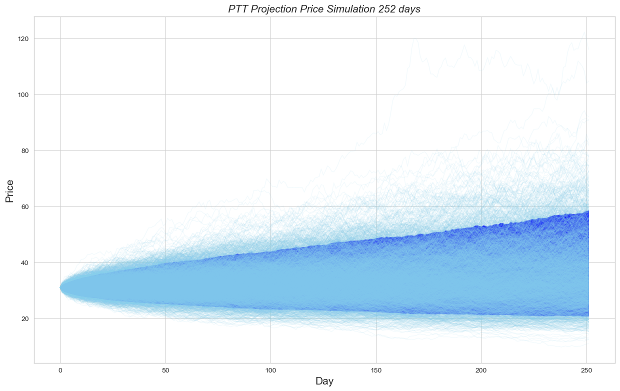

Create a function to generate future day simulations:

import datetime
 
#create future day
start = datetime.datetime.strptime("26-08-2022", "%d-%m-%Y")
end = datetime.datetime.strptime("15-08-2023", "%d-%m-%Y")
date_generated = [start + datetime.timedelta(days=x) for x in range(0, (end - start).days)]
date_generated =  pd.DataFrame(date_generated)
date_generated['day_name'] = date_generated.iloc[:,0].dt.day_name()
date_generated = date_generated[(date_generated['day_name'] != 'Saturday')&(date_generated['day_name'] != 'Sunday')]

price_matrix.index = date_generated.iloc[:,0].values

price_matrix.head()

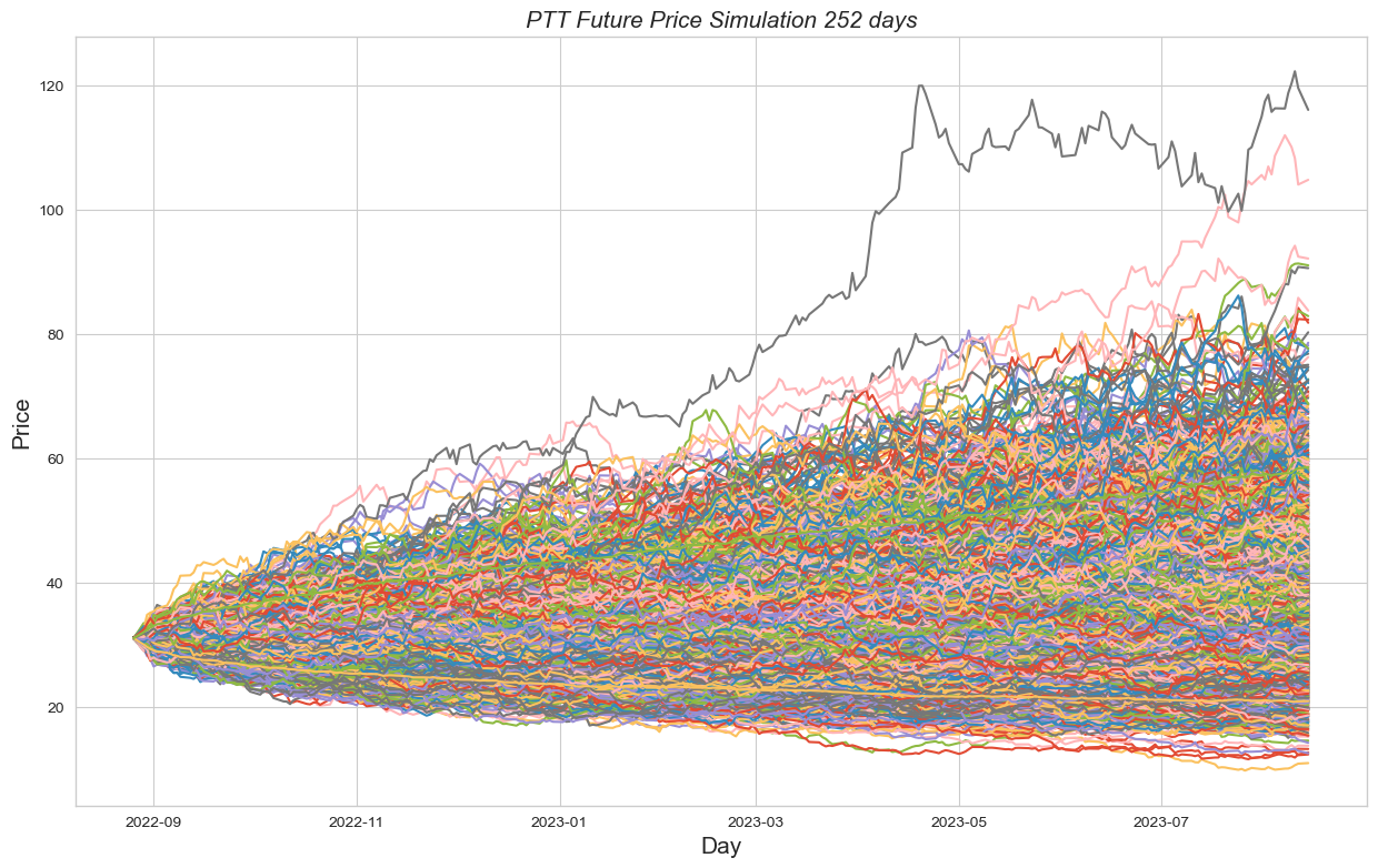
visulization section

plt.plot(price_matrix)
plt.title('PTT Future Price Simulation 252 days', size=15, fontstyle='italic')
plt.xlabel('Day', size=15)
plt.ylabel('Price', size=15)
plt.show()

Conclusion

In conclusion, the Monte Carlo Simulation is a valuable method for estimating the range of possible future stock prices by simulating random future scenarios based on historical data. It helps investors better understand the potential risks and opportunities associated with a particular stock, and can be a useful tool in making informed investment decisions.