
What Idea about heat map chart ?
The code provided uses pandas, matplotlib, and seaborn to create a heatmap chart of the SET index.
It reads a CSV file containing daily SET index data from 1975 to 2021, resamples the data to weekly and monthly periods, and calculates the percentage change for the last ten years.
It then pivots the data to create a matrix where the rows represent years, the columns represent months, and the cells contain the percentage change in the SET index for each month and year.
It also calculates the average percentage change for each year and month and adds them as a row and column to the matrix. Finally, it creates a heatmap using seaborn to visualize the matrix.
Import the necessary libraries and the dataset
import pandas as pd
import numpy as np
import matplotlib.pyplot as plt
import seaborn as sns
import warnings
%matplotlib inline
plt.rcParams["figure.figsize"] = (15,11)
sns.set_style('whitegrid')
warnings.filterwarnings("ignore")
Resample the dataset to weekly and monthly intervals
data = pd.read_csv('SET_Data_from1970-2021.csv',index_col='Date',parse_dates=True)
data| Symbol | Open | High | Low | Close | Volume | |
|---|---|---|---|---|---|---|
| Date | ||||||
| 1975-04-30 | SET | 100.00 | 100.00 | 100.00 | 100.00 | 163310 |
| 1975-05-02 | SET | 99.96 | 99.96 | 99.96 | 99.96 | 150220 |
| 1975-05-06 | SET | 99.53 | 99.53 | 99.53 | 99.53 | 260100 |
| 1975-05-07 | SET | 99.13 | 99.13 | 99.13 | 99.13 | 35480 |
| 1975-05-08 | SET | 97.88 | 97.88 | 97.88 | 97.88 | 52500 |
| … | … | … | … | … | … | … |
| 2021-12-24 | SET | 1642.64 | 1644.12 | 1635.19 | 1637.22 | 21132799040 |
| 2021-12-27 | SET | 1641.28 | 1642.42 | 1632.79 | 1636.50 | 20516253580 |
| 2021-12-28 | SET | 1640.97 | 1650.28 | 1640.61 | 1641.52 | 25104505000 |
| 2021-12-29 | SET | 1643.43 | 1654.98 | 1641.75 | 1653.33 | 24677866340 |
| 2021-12-30 | SET | 1657.29 | 1660.85 | 1652.37 | 1657.62 | 21309077960 |
11452 rows × 6 columns
data.resample('W-Fri').agg({'Open':'first',
                                'High':'max',
                                'Low':'min',
'Close':'last'})| Open | High | Low | Close | |
|---|---|---|---|---|
| Date | ||||
| 1975-05-02 | 100.00 | 100.00 | 99.96 | 99.96 |
| 1975-05-09 | 99.53 | 99.53 | 96.64 | 96.64 |
| 1975-05-16 | 95.37 | 95.37 | 89.45 | 89.45 |
| 1975-05-23 | 87.11 | 91.91 | 85.73 | 91.91 |
| 1975-05-30 | 90.69 | 90.69 | 88.89 | 89.98 |
| … | … | … | … | … |
| 2021-12-03 | 1608.01 | 1617.55 | 1563.04 | 1588.19 |
| 2021-12-10 | 1600.17 | 1623.82 | 1595.14 | 1618.23 |
| 2021-12-17 | 1626.29 | 1646.85 | 1616.51 | 1641.73 |
| 2021-12-24 | 1631.22 | 1645.71 | 1612.96 | 1637.22 |
| 2021-12-31 | 1641.28 | 1660.85 | 1632.79 | 1657.62 |
2436 rows × 4 columns
Calculate the monthly returns for the last ten years and add them to a new dataframe
add monthly return
df_monthly = data.copy()
df_monthly = df_monthly.resample('M').agg({'Open':'first',
                                'High':'max',
                                'Low':'min',
                                'Close':'last'})
df_monthly| Open | High | Low | Close | |
|---|---|---|---|---|
| Date | ||||
| 1975-04-30 | 100.00 | 100.00 | 100.00 | 100.00 |
| 1975-05-31 | 99.96 | 99.96 | 85.73 | 89.98 |
| 1975-06-30 | 89.53 | 91.64 | 89.42 | 91.64 |
| 1975-07-31 | 91.90 | 100.11 | 91.90 | 98.02 |
| 1975-08-31 | 100.00 | 100.00 | 98.14 | 98.39 |
| … | … | … | … | … |
| 2021-08-31 | 1523.42 | 1643.76 | 1512.28 | 1638.75 |
| 2021-09-30 | 1643.01 | 1658.08 | 1591.81 | 1605.68 |
| 2021-10-31 | 1600.59 | 1651.41 | 1593.32 | 1623.43 |
| 2021-11-30 | 1627.59 | 1658.60 | 1565.95 | 1568.69 |
| 2021-12-31 | 1576.26 | 1660.85 | 1563.04 | 1657.62 |
561 rows × 4 columns
type(df_monthly[['Close']])
# use this

pandas.core.frame.DataFramedf_monthly[['Close']]| Close | |
|---|---|
| Date | |
| 1975-04-30 | 100.00 |
| 1975-05-31 | 89.98 |
| 1975-06-30 | 91.64 |
| 1975-07-31 | 98.02 |
| 1975-08-31 | 98.39 |
| … | … |
| 2021-08-31 | 1638.75 |
| 2021-09-30 | 1605.68 |
| 2021-10-31 | 1623.43 |
| 2021-11-30 | 1568.69 |
| 2021-12-31 | 1657.62 |
561 rows × 1 columns
lasttenyear = df_monthly.pct_change().loc['2011':'2021'][['Close']]
lasttenyear| Close | |
|---|---|
| Date | |
| 2011-01-31 | -0.066482 |
| 2011-02-28 | 0.024697 |
| 2011-03-31 | 0.060299 |
| 2011-04-30 | 0.043991 |
| 2011-05-31 | -0.018042 |
| … | … |
| 2021-08-31 | 0.076765 |
| 2021-09-30 | -0.020180 |
| 2021-10-31 | 0.011055 |
| 2021-11-30 | -0.033719 |
| 2021-12-31 | 0.056691 |
132 rows × 1 columns
lasttenyear=lasttenyear.reset_index()lasttenyear['year'] = pd.DatetimeIndex(lasttenyear['Date'] ).yearlasttenyear['month'] = pd.DatetimeIndex(lasttenyear['Date'] ).monthlasttenyear| Date | Close | year | month | |
|---|---|---|---|---|
| 0 | 2011-01-31 | -0.066482 | 2011 | 1 |
| 1 | 2011-02-28 | 0.024697 | 2011 | 2 |
| 2 | 2011-03-31 | 0.060299 | 2011 | 3 |
| 3 | 2011-04-30 | 0.043991 | 2011 | 4 |
| 4 | 2011-05-31 | -0.018042 | 2011 | 5 |
| … | … | … | … | … |
| 127 | 2021-08-31 | 0.076765 | 2021 | 8 |
| 128 | 2021-09-30 | -0.020180 | 2021 | 9 |
| 129 | 2021-10-31 | 0.011055 | 2021 | 10 |
| 130 | 2021-11-30 | -0.033719 | 2021 | 11 |
| 131 | 2021-12-31 | 0.056691 | 2021 | 12 |
132 rows × 4 columns
lasttenyear.Date.apply(lambda x: x.strftime('%b')) 0 Jan
1 Feb
2 Mar
3 Apr
4 May
...
127 Aug
128 Sep
129 Oct
130 Nov
131 Dec
Name: Date, Length: 132, dtype: objectlasttenyear['smonth']= lasttenyear.Date.apply(lambda x: x.strftime('%b'))lasttenyear| Date | Close | year | month | smonth | |
|---|---|---|---|---|---|
| 0 | 2011-01-31 | -0.066482 | 2011 | 1 | Jan |
| 1 | 2011-02-28 | 0.024697 | 2011 | 2 | Feb |
| 2 | 2011-03-31 | 0.060299 | 2011 | 3 | Mar |
| 3 | 2011-04-30 | 0.043991 | 2011 | 4 | Apr |
| 4 | 2011-05-31 | -0.018042 | 2011 | 5 | May |
| … | … | … | … | … | … |
| 127 | 2021-08-31 | 0.076765 | 2021 | 8 | Aug |
| 128 | 2021-09-30 | -0.020180 | 2021 | 9 | Sep |
| 129 | 2021-10-31 | 0.011055 | 2021 | 10 | Oct |
| 130 | 2021-11-30 | -0.033719 | 2021 | 11 | Nov |
| 131 | 2021-12-31 | 0.056691 | 2021 | 12 | Dec |
132 rows × 5 columns
lasttenyear.dtypes Date datetime64[ns]
Close float64
year int64
month int64
smonth object
dtype: objectdf=lasttenyear[['year','month','Close']]df.pivot(index='year',columns='month').Close| month | 1 | 2 | 3 | 4 | 5 | 6 | 7 | 8 | 9 | 10 | 11 | 12 |
|---|---|---|---|---|---|---|---|---|---|---|---|---|
| year | ||||||||||||
| 2011 | -0.066482 | 0.024697 | 0.060299 | 0.043991 | -0.018042 | -0.030126 | 0.088384 | -0.056002 | -0.143769 | 0.063894 | 0.021113 | 0.030131 |
| 2012 | 0.057202 | 0.070971 | 0.030898 | 0.026505 | -0.070811 | 0.026816 | 0.023197 | 0.023497 | 0.058095 | 0.000062 | 0.019378 | 0.051275 |
| 2013 | 0.059105 | 0.045706 | 0.012636 | 0.023574 | -0.022399 | -0.070528 | -0.019809 | -0.090532 | 0.068655 | 0.043176 | -0.049727 | -0.052818 |
| 2014 | -0.018811 | 0.040062 | 0.038428 | 0.028105 | 0.000558 | 0.049459 | 0.011200 | 0.039431 | 0.015394 | -0.000952 | 0.006155 | -0.060380 |
| 2015 | 0.055807 | 0.003643 | -0.051083 | 0.013812 | -0.020102 | 0.005682 | -0.042823 | -0.040073 | -0.024168 | 0.034055 | -0.025263 | -0.052718 |
| 2016 | 0.010062 | 0.024128 | 0.056538 | -0.002195 | 0.014004 | 0.014541 | 0.054727 | 0.015990 | -0.042126 | 0.008434 | 0.009708 | 0.021652 |
| 2017 | 0.022276 | -0.011253 | 0.009971 | -0.005581 | -0.002975 | 0.008376 | 0.000851 | 0.025430 | 0.035269 | 0.028814 | -0.013931 | 0.033180 |
| 2018 | 0.041712 | 0.001790 | -0.029435 | 0.002167 | -0.029852 | -0.076081 | 0.066565 | 0.011629 | 0.020231 | -0.049715 | -0.016350 | -0.047460 |
| 2019 | 0.049780 | 0.007157 | -0.008969 | 0.021280 | -0.031849 | 0.067966 | -0.010616 | -0.033324 | -0.010695 | -0.021824 | -0.006806 | -0.006758 |
| 2020 | -0.041586 | -0.114666 | -0.160132 | 0.156147 | 0.031644 | -0.002845 | -0.007841 | -0.013451 | -0.056170 | -0.034025 | 0.178551 | 0.029141 |
| 2021 | 0.012164 | 0.020314 | 0.060416 | -0.002571 | 0.006607 | -0.003640 | -0.041485 | 0.076765 | -0.020180 | 0.011055 | -0.033719 | 0.056691 |
Display the pivoted dataframe as a heat map chart using the heatmap() function
pivot = df.pivot(index='year',columns='month').Close
pivot.columns = ['Jan','Feb','Mar','Apr','May','Jun','Jul','Aug','Sep','Oct','Nov','Dec']
import seaborn as sns
sns.set(rc = {'figure.figsize':(15,8)})
sns.heatmap(pivot,cmap='RdYlGn',annot=True,fmt='.2%')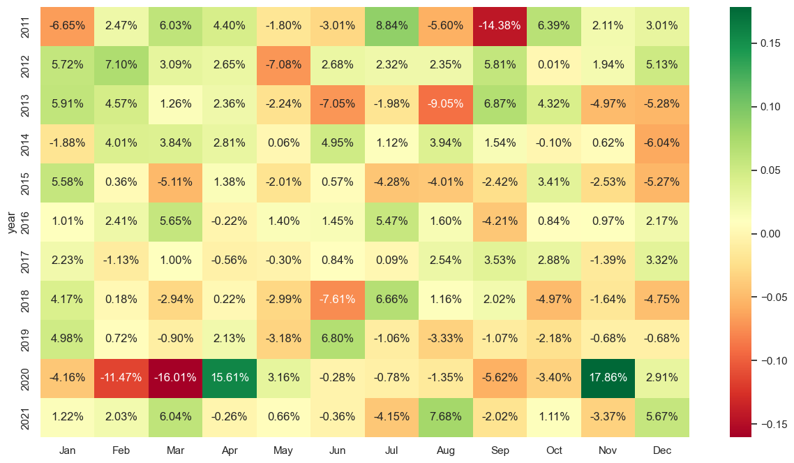
df.groupby('year').mean()
| month | Close | |
|---|---|---|
| year | ||
| 2011 | 6.5 | 0.001507 |
| 2012 | 6.5 | 0.026424 |
| 2013 | 6.5 | -0.004413 |
| 2014 | 6.5 | 0.012387 |
| 2015 | 6.5 | -0.011936 |
| 2016 | 6.5 | 0.015455 |
| 2017 | 6.5 | 0.010869 |
| 2018 | 6.5 | -0.008733 |
| 2019 | 6.5 | 0.001278 |
| 2020 | 6.5 | -0.002936 |
| 2021 | 6.5 | 0.011868 |
pivot['avg']=df.groupby('year').mean()['Close']
Modify the column names to show abbreviated month names and add a column to display the average monthly return for each year
sns.heatmap(pivot,cmap='RdYlGn',annot=True,fmt='.2%')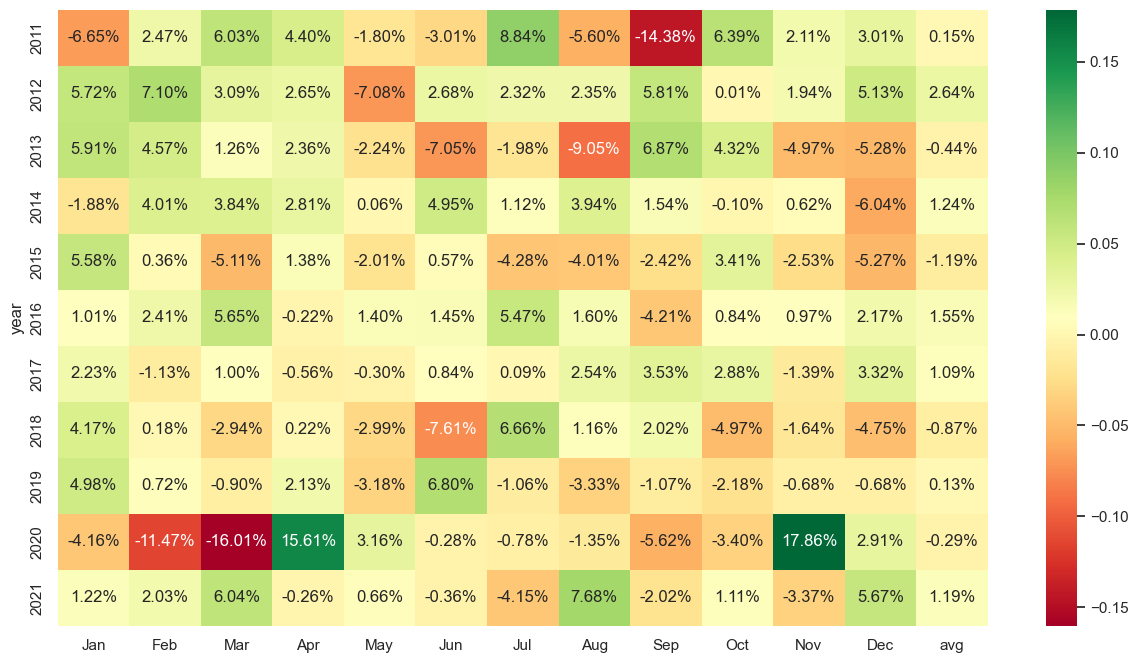
pivot.columns=[1,2,3,4,5,6,7,8,9,10,11,12,'avg']Add a row to show the average monthly return for each month
pivot.loc['mavg']=df.groupby('month').mean()['Close']
pivot| 1 | 2 | 3 | 4 | 5 | 6 | 7 | 8 | 9 | 10 | 11 | 12 | avg | |
|---|---|---|---|---|---|---|---|---|---|---|---|---|---|
| year | |||||||||||||
| 2011 | -0.066482 | 0.024697 | 0.060299 | 0.043991 | -0.018042 | -0.030126 | 0.088384 | -0.056002 | -0.143769 | 0.063894 | 0.021113 | 0.030131 | 0.001507 |
| 2012 | 0.057202 | 0.070971 | 0.030898 | 0.026505 | -0.070811 | 0.026816 | 0.023197 | 0.023497 | 0.058095 | 0.000062 | 0.019378 | 0.051275 | 0.026424 |
| 2013 | 0.059105 | 0.045706 | 0.012636 | 0.023574 | -0.022399 | -0.070528 | -0.019809 | -0.090532 | 0.068655 | 0.043176 | -0.049727 | -0.052818 | -0.004413 |
| 2014 | -0.018811 | 0.040062 | 0.038428 | 0.028105 | 0.000558 | 0.049459 | 0.011200 | 0.039431 | 0.015394 | -0.000952 | 0.006155 | -0.060380 | 0.012387 |
| 2015 | 0.055807 | 0.003643 | -0.051083 | 0.013812 | -0.020102 | 0.005682 | -0.042823 | -0.040073 | -0.024168 | 0.034055 | -0.025263 | -0.052718 | -0.011936 |
| 2016 | 0.010062 | 0.024128 | 0.056538 | -0.002195 | 0.014004 | 0.014541 | 0.054727 | 0.015990 | -0.042126 | 0.008434 | 0.009708 | 0.021652 | 0.015455 |
| 2017 | 0.022276 | -0.011253 | 0.009971 | -0.005581 | -0.002975 | 0.008376 | 0.000851 | 0.025430 | 0.035269 | 0.028814 | -0.013931 | 0.033180 | 0.010869 |
| 2018 | 0.041712 | 0.001790 | -0.029435 | 0.002167 | -0.029852 | -0.076081 | 0.066565 | 0.011629 | 0.020231 | -0.049715 | -0.016350 | -0.047460 | -0.008733 |
| 2019 | 0.049780 | 0.007157 | -0.008969 | 0.021280 | -0.031849 | 0.067966 | -0.010616 | -0.033324 | -0.010695 | -0.021824 | -0.006806 | -0.006758 | 0.001278 |
| 2020 | -0.041586 | -0.114666 | -0.160132 | 0.156147 | 0.031644 | -0.002845 | -0.007841 | -0.013451 | -0.056170 | -0.034025 | 0.178551 | 0.029141 | -0.002936 |
| 2021 | 0.012164 | 0.020314 | 0.060416 | -0.002571 | 0.006607 | -0.003640 | -0.041485 | 0.076765 | -0.020180 | 0.011055 | -0.033719 | 0.056691 | 0.011868 |
| mavg | 0.016475 | 0.010232 | 0.001779 | 0.027749 | -0.013020 | -0.000944 | 0.011123 | -0.003695 | -0.009042 | 0.007543 | 0.008101 | 0.000176 | NaN |
Display the modified heatmap chart using the heatmap() function with the desired settings.
pivot.columns = ['Jan','Feb','Mar','Apr','May','Jun','Jul','Aug','Sep','Oct','Nov','Dec','avg']

sns.heatmap(pivot,cmap='RdYlGn',annot=True,fmt='.2%')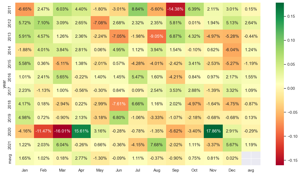
Finally, we plotted the updated pivot table as a heatmap using seaborn library.
The heatmap chart is a graphical representation of data where individual values contained in a matrix are represented as colors. In this case, the heatmap chart is used to visualize the percentage change in the SET index for each month and year. Positive percentage changes are represented with green colors, while negative percentage changes are represented with red colors. The intensity of the color indicates the magnitude of the percentage change. This heatmap can help investors and analysts to identify trends or patterns in the SET index data over the years.
Conclusion
In conclusion, the heat map chart provides an easy and efficient way to visualize data in a clear and concise manner.
The heatmap chart used in this code helps to visualize the SET index’s monthly percentage change for the last ten years, making it easier to understand the SET index’s performance over time.
The addition of the average percentage change for each year and month to the heatmap chart helps to provide further insights into the SET index’s performance.