Mastering Net Advance Volume Analysis with Python: A Comprehensive Guide for Investors

In today’s financial markets, understanding market breadth is essential to gauge the overall market sentiment. Market breadth indicators can help investors and traders make informed decisions by analyzing the underlying strength or weakness of a market. One such indicator is the Net Advance Volume, which takes into account the number of advancing and declining stocks along with their trading volumes.

This code downloads stock data, cleans it, calculates value averages, percent changes, and signs, then groups the data by date and sign, and finally formats the data in a more readable way.

Importing Libraries:

Begin by importing the necessary libraries:

import pandas as pd
import numpy as np
import yfinance as yf

Loading the Data:

 symbol_list_set50
  ['ADVANC.BK',
     'AOT.BK',
     'AWC.BK',
     'BANPU.BK',
     'BBL.BK',
     'BDMS.BK',
     'BEM.BK',
     'BGRIM.BK',
     'BH.BK',
     'BTS.BK',
     'CBG.BK',
     'CENTEL.BK',
     'COM7.BK',
     'CPALL.BK',
     'CPF.BK',
     'CPN.BK',
     'CRC.BK',
     'DELTA.BK',
     'EA.BK',
     'EGCO.BK',
     'GLOBAL.BK',
     'GPSC.BK',
     'GULF.BK',
     'HMPRO.BK',
     'INTUCH.BK',
     'IVL.BK',
     'JMART.BK',
     'JMT.BK',
     'KBANK.BK',
     'KTB.BK',
     'KTC.BK',
     'LH.BK',
     'MINT.BK',
     'MTC.BK',
     'OR.BK',
     'OSP.BK',
     'PTT.BK',
     'PTTEP.BK',
     'PTTGC.BK',
     'RATCH.BK',
     'SAWAD.BK',
     'SCB.BK',
     'SCC.BK',
     'SCGP.BK',
     'TIDLOR.BK',
     'TISCO.BK',
     'TOP.BK',
     'TRUE.BK',
     'TTB.BK',
     'TU.BK']

Download data from the symbol ticker list:

data = yf.download(symbol_list_set50, start='2020-09-01',end='2022-09-01', interval='1d')
    [*********************100%***********************]  50 of 50 completed
data

Cleaning the Data:

data.fillna(method='ffill',inplace=True)
df=data.stack()
stock_df =df.sort_index(level=1)
stock_df.index.names=['Date','Stock']
stock_df

Calculating Value Average:

# should use average price to * volume , or vwap * average price
stock_df['value']=((stock_df['Open']+stock_df['High']+stock_df['Low']+stock_df['Close'])/4)*stock_df['Volume']
stock_df

Calculating Percent Change and Sign:

stock_df['pct_change']=stock_df['Close'].pct_change()
stock_df['sign']=np.sign(stock_df['pct_change'])
stock_df

stock_df.groupby(by=['Date','sign'])['value'].sum().to_frame()

Grouping Data and Calculating AD Volume:

ad_volume_df = stock_df.groupby(by=['Date','sign'])['value'].sum().to_frame('ad_volume').reset_index()
ad_volume_df

Formatting the Data:

In this section, we format the data to make it easier to visualize and analyze. We start by pivoting the data using the ‘ad_volume’ values, and setting the ‘Date’ as the index and ‘sign’ as columns.

ad_volume_df = pd.pivot_table(ad_volume_df,values='ad_volume',index=['Date'],columns='sign')
ad_volume_df

This creates a DataFrame ‘ad_volume_df’ with the columns -1.0, 0.0, and 1.0 representing declining volume, unchanged volume, and advancing volume, respectively.

Next, we rename the columns to make them more descriptive: ‘Vol_decline’ for -1.0, ‘Vol_unchanged’ for 0.0, and ‘Vol_advance’ for 1.0.

ad_volume_df = ad_volume_df.rename(columns={-1.0:'Vol_decline',0.0:'Vol_unchanged',1.0:'Vol_advance'})
ad_volume_df

We then calculate the ‘net_ad_volume’ by subtracting the declining volume from the advancing volume and add a new column ‘AD_Volume_line’, which is the cumulative sum of the ‘net_ad_volume’ column. Finally, we reset the index of the DataFrame.

ad_volume_df['net_ad_volume'] = ad_volume_df['Vol_advance']- ad_volume_df['Vol_decline']
ad_volume_df['AD_Volume_line']=ad_volume_df['net_ad_volume'].cumsum()
ad_volume_df=ad_volume_df.reset_index()
ad_volume_df

Now, we create a bar chart using the Plotly library to visualize the Net Advance Volume over time.

fig = px.bar(ad_volume_df,y='net_ad_volume',
             x='Date',template='simple_white',
             barmode='relative',
             title='Market Breadth : Net Advance Volume')
fig.update_xaxes(rangebreaks=[dict(bounds=['sat','mo'])])
fig.update_xaxes(rangeslider_visible=True)
fig.show()

visualize the Advance-Decline Volume data to understand market trends. By creating bar charts, line charts, and bubble charts (if needed), we can analyze the market breadth and make more informed decisions based on the Net Advance Volume. This analysis can be a valuable tool for traders and investors to gauge market sentiment and identify potential opportunities.

Print the index of the data DataFrame, showing the dates included in the dataset.

data.index

    DatetimeIndex(['2020-09-01', '2020-09-02', '2020-09-03', '2020-09-08',
                   '2020-09-09', '2020-09-10', '2020-09-11', '2020-09-14',
                   '2020-09-15', '2020-09-16',
                   ...
                   '2022-08-18', '2022-08-19', '2022-08-22', '2022-08-23',
                   '2022-08-24', '2022-08-25', '2022-08-26', '2022-08-29',
                   '2022-08-30', '2022-08-31'],
                  dtype='datetime64[ns]', name='Date', length=480, freq=None)

Print the ‘Date’ column of the ad_volume_df DataFrame, showing the dates included in this dataset.

ad_volume_df['Date']
# check you date range
    0     2020-09-01
    1     2020-09-02
    2     2020-09-03
    3     2020-09-08
    4     2020-09-09
             ...    
    475   2022-08-25
    476   2022-08-26
    477   2022-08-29
    478   2022-08-30
    479   2022-08-31
    Name: Date, Length: 480, dtype: datetime64[ns]

Calculate the difference between a complete date range from ‘2020-09-01’ to ‘2022-08-31’ and the dates in data.index. This will show the dates without data.

pd.date_range(start='2020-09-01',end='2022-08-31').difference(data.index)
# will show date with out data
DatetimeIndex(['2020-09-04', '2020-09-05', '2020-09-06', '2020-09-07',
                   '2020-09-12', '2020-09-13', '2020-09-19', '2020-09-20',
                   '2020-09-26', '2020-09-27',
                   ...
                   '2022-07-31', '2022-08-06', '2022-08-07', '2022-08-12',
                   '2022-08-13', '2022-08-14', '2022-08-20', '2022-08-21',
                   '2022-08-27', '2022-08-28'],
                  dtype='datetime64[ns]', length=250, freq=None)

Calculate the difference between a complete date range from ‘2020-09-01’ to ‘2022-08-31’ and the dates in ad_volume_df[‘Date’]. Store the result in a variable called df_break.

df_break=pd.date_range(start='2020-09-01',end='2022-08-31').difference(ad_volume_df['Date'])

Create a line chart using the Plotly library to visualize the ‘AD_Volume_line’ column of the ad_volume_df DataFrame. Update the x-axis range breaks using the df_break variable.

fig = px.line(ad_volume_df,y='AD_Volume_line',
             x='Date',template='simple_white',
             title='Market Breadth : Net Advance Volume')
fig.update_xaxes(rangebreaks=[dict(values=df_break)])
fig.update_xaxes(rangeslider_visible=True)
fig.show()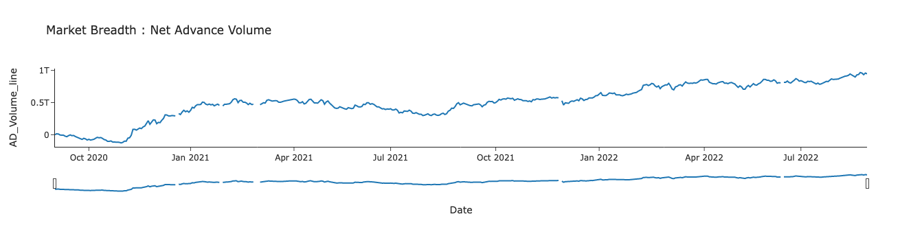

Extract a specific date range from the ad_volume_df DataFrame (between ‘2021-11-25’ and ‘2021-12-05’) by setting the ‘Date’ as the index and using the loc function.

ad_volume_df.set_index('Date').loc['2021-11-25':'2021-12-05']

Create a line chart using the Plotly library to visualize the ‘AD_Volume_line’ column of the ad_volume_df DataFrame for the specific date range mentioned earlier. Update the x-axis range breaks using the df_break variable.

fig = px.line(ad_volume_df,y='AD_Volume_line',
             x='Date',template='simple_white',
             title='Market Breadth : Net Advance Volume')
fig.update_xaxes(rangebreaks=[dict(values=df_break)])
fig.update_xaxes(rangeslider_visible=True)
fig.show()

This will create a bar chart that plots the Net Advance Volume, helping us visualize and analyze market trends.

Conclusion

In conclusion, this article demonstrates how to analyze market trends using the Net Advance Volume, a market breadth indicator that helps investors understand the overall market sentiment. By utilizing Python and its powerful libraries like Pandas and Plotly, we can efficiently handle large datasets and create insightful visualizations, such as line charts, to better comprehend market dynamics.

The step-by-step guide showcases how to process the raw data, manipulate it to calculate the Net Advance Volume, and visualize it using interactive line charts. The ability to visualize and analyze market trends is essential for investors to make informed decisions based on the prevailing market conditions.

By understanding market breadth indicators like the Net Advance Volume, investors can gain valuable insights into the overall strength or weakness of the market, helping them identify potential investment opportunities and develop effective trading strategies.