
What Idea about Stock Analysis and Predicting chart ?
Introduction: In this article, we will explore how to perform stock analysis using Python. We will import and merge multiple datasets, including historical stock prices, earnings per share (EPS), and GDP data. We will then use linear regression to predict stock returns based on historical data. Finally, we will visualize the results using various libraries like pandas, matplotlib, numpy, and seaborn.
importing the necessary libraries
import pandas as pd
import matplotlib.pyplot as plt
import numpy as np
import seaborn as sns
Import Dataframe from Excel
Now, we will read the data from Excel files and store them in pandas DataFrames:
data_set = pd.read_excel('set.xlsx',index_col=0)
data_set_eps = pd.read_excel('set_eps.xlsx',index_col=0)
data_gdpq = pd.read_excel('gdpq.xlsx',engine= 'openpyxl',index_col=0)
After importing the data, we can display the DataFrames to see what they look like:
data_setwe will see dataframe like this
| Prior | Open | High | Low | Close | PE | |
|---|---|---|---|---|---|---|
| Date | ||||||
| 2016-01-04 | 1288.02 | 1286.29 | 1286.36 | 1260.96 | 1263.41 | 22.12 |
| 2016-01-05 | 1263.41 | 1267.20 | 1270.07 | 1251.87 | 1253.34 | 21.99 |
| 2016-01-06 | 1253.34 | 1249.82 | 1260.88 | 1247.89 | 1260.04 | 22.10 |
| 2016-01-07 | 1260.04 | 1237.81 | 1244.04 | 1224.83 | 1224.83 | 21.46 |
| 2016-01-08 | 1224.83 | 1232.31 | 1246.70 | 1228.18 | 1244.18 | 21.81 |
| … | … | … | … | … | … | … |
| 2021-10-28 | 1627.61 | 1626.27 | 1632.30 | 1622.56 | 1624.31 | 20.81 |
| 2021-10-29 | 1624.31 | 1627.01 | 1629.25 | 1619.14 | 1623.43 | 21.02 |
| 2021-11-01 | 1623.43 | 1627.54 | 1632.73 | 1611.39 | 1613.78 | 20.89 |
| 2021-11-02 | 1613.78 | 1616.86 | 1621.69 | 1608.64 | 1617.89 | 20.96 |
| 2021-11-03 | 1617.89 | 1620.90 | 1623.08 | 1607.72 | 1611.92 | 20.87 |
1422 rows × 6 columns
data_set_eps| Prior | Open | High | Low | Close | PE | EPS | |
|---|---|---|---|---|---|---|---|
| Date | |||||||
| 2021-11-03 | 1617.89 | 1620.90 | 1623.08 | 1607.72 | 1611.92 | 19.3909 | 83.1235 |
| 2021-11-02 | 1613.78 | 1616.86 | 1621.69 | 1608.64 | 1617.89 | 19.4637 | 83.1246 |
| 2021-11-01 | 1623.43 | 1627.54 | 1632.73 | 1611.39 | 1613.78 | 19.4140 | 83.1221 |
| 2021-10-29 | 1624.31 | 1627.01 | 1629.25 | 1619.14 | 1623.43 | 19.5307 | 83.1111 |
| 2021-10-28 | 1627.61 | 1626.27 | 1632.30 | 1622.56 | 1624.31 | 19.5438 | 83.6187 |
| … | … | … | … | … | … | … | … |
| NaT | NaN | NaN | NaN | NaN | NaN | NaN | 54.6940 |
| NaT | NaN | NaN | NaN | NaN | NaN | NaN | 54.6926 |
| NaT | NaN | NaN | NaN | NaN | NaN | NaN | 54.6938 |
| NaT | NaN | NaN | NaN | NaN | NaN | NaN | 54.6979 |
| NaT | NaN | NaN | NaN | NaN | NaN | NaN | 54.6952 |
3088 rows × 7 columns
data_gdpq| GDP | |
|---|---|
| Date | |
| 2016-03-31 | 3597737000000 |
| 2016-06-30 | 3557050000000 |
| 2016-09-30 | 3628315000000 |
| 2016-12-31 | 3807235000000 |
| 2017-03-31 | 3830606000000 |
| 2017-06-30 | 3753348000000 |
| 2017-09-30 | 3854593000000 |
| 2017-12-31 | 4050117000000 |
| 2018-03-31 | 4051915000000 |
| 2018-06-30 | 3998560000000 |
| 2018-09-30 | 4063764000000 |
| 2018-12-31 | 4254466000000 |
| 2019-03-31 | 4223706000000 |
| 2019-06-30 | 4156001000000 |
| 2019-09-30 | 4181774000000 |
| 2019-12-31 | 4336605000000 |
| 2020-03-31 | 4158483000000 |
| 2020-06-30 | 3545622000000 |
| 2020-09-30 | 3860959000000 |
| 2020-12-31 | 4133222000000 |
| 2021-03-31 | 4070526000000 |
| 2021-06-30 | 3923731000000 |
1422 rows × 7 columns
Merging DataFrames
We will now merge the data between data_set and data_set_eps DataFrames:
min_date = data_set_eps.index.min()
max_date = data_set_eps.index.max()
date_range = (min_date, max_date)
date_range
(Timestamp('2016-01-04 00:00:00'), Timestamp('2021-11-03 00:00:00'))data_set_eps_subset = data_set_eps.loc[data_set.index, ["PE", "EPS"]]
df1 = pd.merge(data_set, data_set_eps_subset, how="left", left_index=True, right_index=True)data_set_eps_subset| PE | EPS | |
|---|---|---|
| Date | ||
| 2016-01-04 | 17.3305 | 72.2368 |
| 2016-01-05 | 17.1919 | 72.2431 |
| 2016-01-06 | 17.2866 | 72.2438 |
| 2016-01-07 | 16.8012 | 72.2363 |
| 2016-01-08 | 17.0010 | 72.2296 |
| … | … | … |
| 2021-10-28 | 19.5438 | 83.6187 |
| 2021-10-29 | 19.5307 | 83.1111 |
| 2021-11-01 | 19.4140 | 83.1221 |
| 2021-11-02 | 19.4637 | 83.1246 |
| 2021-11-03 | 19.3909 | 83.1235 |
1422 rows × 2 columns
df1| Prior | Open | High | Low | Close | PE_x | PE_y | EPS | |
|---|---|---|---|---|---|---|---|---|
| Date | ||||||||
| 2016-01-04 | 1288.02 | 1286.29 | 1286.36 | 1260.96 | 1263.41 | 22.12 | 17.3305 | 72.2368 |
| 2016-01-05 | 1263.41 | 1267.20 | 1270.07 | 1251.87 | 1253.34 | 21.99 | 17.1919 | 72.2431 |
| 2016-01-06 | 1253.34 | 1249.82 | 1260.88 | 1247.89 | 1260.04 | 22.10 | 17.2866 | 72.2438 |
| 2016-01-07 | 1260.04 | 1237.81 | 1244.04 | 1224.83 | 1224.83 | 21.46 | 16.8012 | 72.2363 |
| 2016-01-08 | 1224.83 | 1232.31 | 1246.70 | 1228.18 | 1244.18 | 21.81 | 17.0010 | 72.2296 |
| … | … | … | … | … | … | … | … | … |
| 2021-10-28 | 1627.61 | 1626.27 | 1632.30 | 1622.56 | 1624.31 | 20.81 | 19.5438 | 83.6187 |
| 2021-10-29 | 1624.31 | 1627.01 | 1629.25 | 1619.14 | 1623.43 | 21.02 | 19.5307 | 83.1111 |
| 2021-11-01 | 1623.43 | 1627.54 | 1632.73 | 1611.39 | 1613.78 | 20.89 | 19.4140 | 83.1221 |
| 2021-11-02 | 1613.78 | 1616.86 | 1621.69 | 1608.64 | 1617.89 | 20.96 | 19.4637 | 83.1246 |
| 2021-11-03 | 1617.89 | 1620.90 | 1623.08 | 1607.72 | 1611.92 | 20.87 | 19.3909 | 83.1235 |
1422 rows × 8 columns
Adding GDP Data to the Merged DataFrame
Next, we will add the GDP data to the merged DataFrame
data_gdpq.index.year

Int64Index([2016, 2016, 2016, 2016, 2017, 2017, 2017, 2017, 2018, 2018, 2018,2018, 2019, 2019, 2019, 2019, 2020, 2020, 2020, 2020, 2021, 2021],
dtype='int64', name='Date')data_gdpq.groupby(data_gdpq.index.year)['GDP'].mean()
Date
2016 3.647584e+12
2017 3.872166e+12
2018 4.092176e+12
2019 4.224522e+12
2020 3.924572e+12
2021 3.997128e+12
Name: GDP, dtype: float64gdp_yearly = data_gdpq.groupby(data_gdpq.index.year)['GDP'].mean()
for i in range(2016,2022):
df1.loc[str(i),'gdp'] = gdp_yearly.loc[i]df1| Prior | Open | High | Low | Close | PE_x | PE_y | EPS | gdp | |
|---|---|---|---|---|---|---|---|---|---|
| Date | |||||||||
| 2016-01-04 | 1288.02 | 1286.29 | 1286.36 | 1260.96 | 1263.41 | 22.12 | 17.3305 | 72.2368 | 3.647584e+12 |
| 2016-01-05 | 1263.41 | 1267.20 | 1270.07 | 1251.87 | 1253.34 | 21.99 | 17.1919 | 72.2431 | 3.647584e+12 |
| 2016-01-06 | 1253.34 | 1249.82 | 1260.88 | 1247.89 | 1260.04 | 22.10 | 17.2866 | 72.2438 | 3.647584e+12 |
| 2016-01-07 | 1260.04 | 1237.81 | 1244.04 | 1224.83 | 1224.83 | 21.46 | 16.8012 | 72.2363 | 3.647584e+12 |
| 2016-01-08 | 1224.83 | 1232.31 | 1246.70 | 1228.18 | 1244.18 | 21.81 | 17.0010 | 72.2296 | 3.647584e+12 |
| … | … | … | … | … | … | … | … | … | … |
| 2021-10-28 | 1627.61 | 1626.27 | 1632.30 | 1622.56 | 1624.31 | 20.81 | 19.5438 | 83.6187 | 3.997128e+12 |
| 2021-10-29 | 1624.31 | 1627.01 | 1629.25 | 1619.14 | 1623.43 | 21.02 | 19.5307 | 83.1111 | 3.997128e+12 |
| 2021-11-01 | 1623.43 | 1627.54 | 1632.73 | 1611.39 | 1613.78 | 20.89 | 19.4140 | 83.1221 | 3.997128e+12 |
| 2021-11-02 | 1613.78 | 1616.86 | 1621.69 | 1608.64 | 1617.89 | 20.96 | 19.4637 | 83.1246 | 3.997128e+12 |
| 2021-11-03 | 1617.89 | 1620.90 | 1623.08 | 1607.72 | 1611.92 | 20.87 | 19.3909 | 83.1235 | 3.997128e+12 |
1422 rows × 9 columns
Calculating and Adding Stock Return to the DataFrame
We will now calculate the daily stock return and add it to the DataFrame
df1['Return_shift'] = df1.Close.pct_change()df1.dropna(inplace=True)df1| Prior | Open | High | Low | Close | PE_x | PE_y | EPS | gdp | Return_shift | |
|---|---|---|---|---|---|---|---|---|---|---|
| Date | ||||||||||
| 2016-01-05 | 1263.41 | 1267.20 | 1270.07 | 1251.87 | 1253.34 | 21.99 | 17.1919 | 72.2431 | 3.647584e+12 | -0.007970 |
| 2016-01-06 | 1253.34 | 1249.82 | 1260.88 | 1247.89 | 1260.04 | 22.10 | 17.2866 | 72.2438 | 3.647584e+12 | 0.005346 |
| 2016-01-07 | 1260.04 | 1237.81 | 1244.04 | 1224.83 | 1224.83 | 21.46 | 16.8012 | 72.2363 | 3.647584e+12 | -0.027944 |
| 2016-01-08 | 1224.83 | 1232.31 | 1246.70 | 1228.18 | 1244.18 | 21.81 | 17.0010 | 72.2296 | 3.647584e+12 | 0.015798 |
| 2016-01-11 | 1244.18 | 1233.80 | 1235.18 | 1220.96 | 1234.50 | 21.63 | 16.8695 | 72.2242 | 3.647584e+12 | -0.007780 |
| … | … | … | … | … | … | … | … | … | … | … |
| 2021-10-28 | 1627.61 | 1626.27 | 1632.30 | 1622.56 | 1624.31 | 20.81 | 19.5438 | 83.6187 | 3.997128e+12 | -0.002028 |
| 2021-10-29 | 1624.31 | 1627.01 | 1629.25 | 1619.14 | 1623.43 | 21.02 | 19.5307 | 83.1111 | 3.997128e+12 | -0.000542 |
| 2021-11-01 | 1623.43 | 1627.54 | 1632.73 | 1611.39 | 1613.78 | 20.89 | 19.4140 | 83.1221 | 3.997128e+12 | -0.005944 |
| 2021-11-02 | 1613.78 | 1616.86 | 1621.69 | 1608.64 | 1617.89 | 20.96 | 19.4637 | 83.1246 | 3.997128e+12 | 0.002547 |
| 2021-11-03 | 1617.89 | 1620.90 | 1623.08 | 1607.72 | 1611.92 | 20.87 | 19.3909 | 83.1235 | 3.997128e+12 | -0.003690 |
1421 rows × 10 columns
df1.loc[(df1.EPS>70)& (df1.EPS<80)]| Prior | Open | High | Low | Close | PE_x | PE_y | EPS | gdp | Return_shift | PE_Label | |
|---|---|---|---|---|---|---|---|---|---|---|---|
| Date | |||||||||||
| 2016-01-05 | 1263.41 | 1267.20 | 1270.07 | 1251.87 | 1253.34 | 21.99 | 17.1919 | 72.2431 | 3.647584e+12 | -0.007970 | 1 |
| 2016-01-06 | 1253.34 | 1249.82 | 1260.88 | 1247.89 | 1260.04 | 22.10 | 17.2866 | 72.2438 | 3.647584e+12 | 0.005346 | 1 |
| 2016-01-07 | 1260.04 | 1237.81 | 1244.04 | 1224.83 | 1224.83 | 21.46 | 16.8012 | 72.2363 | 3.647584e+12 | -0.027944 | 1 |
| 2016-01-08 | 1224.83 | 1232.31 | 1246.70 | 1228.18 | 1244.18 | 21.81 | 17.0010 | 72.2296 | 3.647584e+12 | 0.015798 | 1 |
| 2016-01-11 | 1244.18 | 1233.80 | 1235.18 | 1220.96 | 1234.50 | 21.63 | 16.8695 | 72.2242 | 3.647584e+12 | -0.007780 | 1 |
| … | … | … | … | … | … | … | … | … | … | … | … |
| 2016-05-18 | 1406.57 | 1407.66 | 1410.04 | 1399.36 | 1400.50 | 21.16 | 19.3878 | 74.2615 | 3.647584e+12 | -0.004315 | 1 |
| 2016-05-19 | 1400.50 | 1399.39 | 1400.97 | 1384.12 | 1385.86 | 20.94 | 19.1851 | 74.2568 | 3.647584e+12 | -0.010453 | 1 |
| 2016-05-23 | 1385.86 | 1387.81 | 1388.88 | 1377.65 | 1381.69 | 20.88 | 19.1272 | 74.2602 | 3.647584e+12 | -0.003009 | 1 |
| 2016-05-24 | 1381.69 | 1381.54 | 1386.15 | 1376.74 | 1384.26 | 20.92 | 19.1611 | 74.2644 | 3.647584e+12 | 0.001860 | 1 |
| 2016-05-25 | 1384.26 | 1394.65 | 1398.35 | 1390.19 | 1397.63 | 21.13 | 19.3460 | 74.3830 | 3.647584e+12 | 0.009659 | 1 |
93 rows × 11 columns
df1.loc[ (df1.EPS>35)&(df1.EPS<40)]| Prior | Open | High | Low | Close | PE_x | PE_y | EPS | gdp | Return_shift | PE_Label | |
|---|---|---|---|---|---|---|---|---|---|---|---|
| Date | |||||||||||
| 2020-12-03 | 1417.95 | 1424.31 | 1439.22 | 1420.69 | 1438.32 | 28.49 | 26.2152 | 38.9297 | 3.924572e+12 | 0.014366 | 2 |
| 2020-12-04 | 1438.32 | 1439.14 | 1454.94 | 1439.14 | 1449.83 | 28.73 | 26.4263 | 38.9327 | 3.924572e+12 | 0.008002 | 2 |
| 2020-12-08 | 1449.83 | 1447.71 | 1484.73 | 1442.65 | 1478.92 | 29.34 | 26.9521 | 38.9373 | 3.924572e+12 | 0.020064 | 2 |
| 2020-12-09 | 1478.92 | 1491.67 | 1503.89 | 1474.83 | 1482.67 | 29.41 | 27.0420 | 38.9369 | 3.924572e+12 | 0.002536 | 2 |
| 2020-12-14 | 1482.67 | 1490.79 | 1495.18 | 1471.56 | 1476.13 | 29.28 | 26.9259 | 38.9370 | 3.924572e+12 | -0.004411 | 2 |
| … | … | … | … | … | … | … | … | … | … | … | … |
| 2021-03-05 | 1534.11 | 1530.05 | 1553.92 | 1529.83 | 1544.11 | 40.32 | 39.5819 | 39.0209 | 3.997128e+12 | 0.006518 | 6 |
| 2021-03-08 | 1544.11 | 1558.79 | 1562.56 | 1540.64 | 1543.76 | 40.29 | 39.5730 | 39.0214 | 3.997128e+12 | -0.000227 | 6 |
| 2021-03-09 | 1543.76 | 1551.57 | 1554.96 | 1537.23 | 1550.59 | 40.44 | 39.7479 | 39.0213 | 3.997128e+12 | 0.004424 | 6 |
| 2021-03-10 | 1550.59 | 1553.23 | 1573.55 | 1550.45 | 1573.05 | 41.00 | 40.3238 | 39.0213 | 3.997128e+12 | 0.014485 | 6 |
| 2021-03-11 | 1573.05 | 1583.13 | 1584.61 | 1569.87 | 1575.13 | 41.07 | 40.3772 | 39.0857 | 3.997128e+12 | 0.001322 | 6 |
64 rows × 11 columns
df1.loc[ (df1.EPS>100)]| Prior | Open | High | Low | Close | PE_x | PE_y | EPS | gdp | Return_shift | PE_Label | |
|---|---|---|---|---|---|---|---|---|---|---|---|
| Date | |||||||||||
| 2018-04-02 | 1776.26 | 1775.24 | 1783.73 | 1771.58 | 1782.28 | 18.35 | 17.9799 | 101.0242 | 4.092176e+12 | 0.003389 | 1 |
| 2018-04-03 | 1782.28 | 1774.45 | 1779.04 | 1764.18 | 1765.24 | 18.17 | 17.8016 | 101.0231 | 4.092176e+12 | -0.009561 | 1 |
| 2018-04-04 | 1765.24 | 1766.67 | 1771.58 | 1724.90 | 1724.98 | 17.75 | 17.3944 | 101.0234 | 4.092176e+12 | -0.022807 | 1 |
| 2018-04-05 | 1724.98 | 1735.58 | 1740.84 | 1724.88 | 1739.92 | 17.90 | 17.5470 | 101.0272 | 4.092176e+12 | 0.008661 | 1 |
| 2018-04-09 | 1739.92 | 1736.54 | 1752.91 | 1735.38 | 1751.27 | 18.03 | 17.6620 | 101.0266 | 4.092176e+12 | 0.006523 | 1 |
| … | … | … | … | … | … | … | … | … | … | … | … |
| 2018-08-10 | 1722.48 | 1718.40 | 1719.03 | 1705.20 | 1705.96 | 17.32 | 16.9411 | 105.4328 | 4.092176e+12 | -0.009591 | 1 |
| 2018-08-21 | 1701.42 | 1703.79 | 1707.63 | 1688.59 | 1694.63 | 16.83 | 16.8285 | 100.6324 | 4.092176e+12 | -0.003991 | 1 |
| 2018-08-22 | 1694.63 | 1696.96 | 1705.91 | 1695.34 | 1698.30 | 16.89 | 16.8666 | 100.6112 | 4.092176e+12 | 0.002166 | 1 |
| 2018-10-09 | 1696.22 | 1700.55 | 1708.72 | 1690.92 | 1696.92 | 16.73 | 16.0854 | 105.4485 | 4.092176e+12 | 0.000413 | 1 |
| 2018-10-10 | 1696.92 | 1709.19 | 1721.82 | 1707.63 | 1721.82 | 16.98 | 16.3222 | 105.4503 | 4.092176e+12 | 0.014674 | 1 |
92 rows × 11 columns
Create label for ML training
def pe(pe):
    if pe <=20:
        return 1
    elif (pe>20)&(pe<=28):
        return 2
    elif (pe>28)&(pe<=30):
        return 3
    elif (pe > 30) & (pe <= 34):
        return 4
    elif (pe > 34) & (pe <= 38):
        return 5
    elif (pe > 38) & (pe <= 42):
        return 6
    elif pe > 42:
        return 7
def eps(eps):
if eps <=40:
return 1
elif (eps>40)&(eps<=50):
return 2
elif (eps>50)&(eps<=60):
return 3
elif (eps > 60) & (eps <= 70):
return 4
elif (eps > 70) & (eps <= 80):
return 5
elif (eps > 80) & (eps <= 90):
return 6
elif (eps > 90) & (eps <= 100):
return 7
elif eps > 100 :
return 8def gdp(gdp):
if gdp <=3.750000e+12:
return 1
elif (gdp>3.750000e+12)&(gdp<=4.000000e+12):
return 2
elif (gdp>4.000000e+12)&(gdp<=4.250000e+12):
return 3
elif eps > 4.250000e+12 :
return 4
df1['PE_Label'] = df1['PE_y'].apply(pe)df1['EPS_Label'] = df1['EPS'].apply(eps)df1['GDP_Label'] = df1['gdp'].apply(gdp)df1| Prior | Open | High | Low | Close | PE_x | PE_y | EPS | gdp | Return_shift | PE_Label | EPS_Label | GDP_Label | |
|---|---|---|---|---|---|---|---|---|---|---|---|---|---|
| Date | |||||||||||||
| 2016-01-05 | 1263.41 | 1267.20 | 1270.07 | 1251.87 | 1253.34 | 21.99 | 17.1919 | 72.2431 | 3.647584e+12 | -0.007970 | 1 | 5 | 1 |
| 2016-01-06 | 1253.34 | 1249.82 | 1260.88 | 1247.89 | 1260.04 | 22.10 | 17.2866 | 72.2438 | 3.647584e+12 | 0.005346 | 1 | 5 | 1 |
| 2016-01-07 | 1260.04 | 1237.81 | 1244.04 | 1224.83 | 1224.83 | 21.46 | 16.8012 | 72.2363 | 3.647584e+12 | -0.027944 | 1 | 5 | 1 |
| 2016-01-08 | 1224.83 | 1232.31 | 1246.70 | 1228.18 | 1244.18 | 21.81 | 17.0010 | 72.2296 | 3.647584e+12 | 0.015798 | 1 | 5 | 1 |
| 2016-01-11 | 1244.18 | 1233.80 | 1235.18 | 1220.96 | 1234.50 | 21.63 | 16.8695 | 72.2242 | 3.647584e+12 | -0.007780 | 1 | 5 | 1 |
| … | … | … | … | … | … | … | … | … | … | … | … | … | … |
| 2021-10-28 | 1627.61 | 1626.27 | 1632.30 | 1622.56 | 1624.31 | 20.81 | 19.5438 | 83.6187 | 3.997128e+12 | -0.002028 | 1 | 6 | 2 |
| 2021-10-29 | 1624.31 | 1627.01 | 1629.25 | 1619.14 | 1623.43 | 21.02 | 19.5307 | 83.1111 | 3.997128e+12 | -0.000542 | 1 | 6 | 2 |
| 2021-11-01 | 1623.43 | 1627.54 | 1632.73 | 1611.39 | 1613.78 | 20.89 | 19.4140 | 83.1221 | 3.997128e+12 | -0.005944 | 1 | 6 | 2 |
| 2021-11-02 | 1613.78 | 1616.86 | 1621.69 | 1608.64 | 1617.89 | 20.96 | 19.4637 | 83.1246 | 3.997128e+12 | 0.002547 | 1 | 6 | 2 |
| 2021-11-03 | 1617.89 | 1620.90 | 1623.08 | 1607.72 | 1611.92 | 20.87 | 19.3909 | 83.1235 | 3.997128e+12 | -0.003690 | 1 | 6 | 2 |
1421 rows × 13 columns
Data Preparation:
First, we need to split our dataset into training and testing sets. The training set will be used to train our model, while the testing set will be used to evaluate its performance.
X = df1[['EPS','PE_y','gdp','EPS_Label', 'PE_Label','GDP_Label']]
y = df1['Return_shift']
X_train = X.iloc[:1000]
y_train = y.iloc[:1000]
X_test = X.iloc[1000:1200]
y_test = y.iloc[1000:1200]X_train| EPS | PE_y | gdp | EPS_Label | PE_Label | GDP_Label | |
|---|---|---|---|---|---|---|
| Date | ||||||
| 2016-01-05 | 72.2431 | 17.1919 | 3.647584e+12 | 5 | 1 | 1 |
| 2016-01-06 | 72.2438 | 17.2866 | 3.647584e+12 | 5 | 1 | 1 |
| 2016-01-07 | 72.2363 | 16.8012 | 3.647584e+12 | 5 | 1 | 1 |
| 2016-01-08 | 72.2296 | 17.0010 | 3.647584e+12 | 5 | 1 | 1 |
| 2016-01-11 | 72.2242 | 16.8695 | 3.647584e+12 | 5 | 1 | 1 |
| … | … | … | … | … | … | … |
| 2020-01-29 | 87.4341 | 17.4639 | 3.924572e+12 | 6 | 1 | 2 |
| 2020-01-30 | 87.4127 | 17.4568 | 3.924572e+12 | 6 | 1 | 2 |
| 2020-01-31 | 87.4291 | 17.3440 | 3.924572e+12 | 6 | 1 | 2 |
| 2020-02-03 | 87.3809 | 17.1378 | 3.924572e+12 | 6 | 1 | 2 |
| 2020-02-04 | 87.3742 | 17.4058 | 3.924572e+12 | 6 | 1 | 2 |
1000 rows × 6 columns
y_train
    Date
    2016-01-05   -0.007970
    2016-01-06    0.005346
    2016-01-07   -0.027944
    2016-01-08    0.015798
    2016-01-11   -0.007780
                    ...
    2020-01-29    0.007487
    2020-01-30   -0.000394
    2020-01-31   -0.006463
    2020-02-03   -0.011941
    2020-02-04    0.015588
Name: Return_shift, Length: 1000, dtype: float64X_test| EPS | PE_y | gdp | EPS_Label | PE_Label | GDP_Label | |
|---|---|---|---|---|---|---|
| Date | ||||||
| 2020-02-05 | 87.3689 | 17.5751 | 3.924572e+12 | 6 | 1 | 2 |
| 2020-02-06 | 87.3775 | 17.5939 | 3.924572e+12 | 6 | 1 | 2 |
| 2020-02-07 | 87.3785 | 17.5876 | 3.924572e+12 | 6 | 1 | 2 |
| 2020-02-11 | 87.3733 | 17.4579 | 3.924572e+12 | 6 | 1 | 2 |
| 2020-02-12 | 87.3735 | 17.6405 | 3.924572e+12 | 6 | 1 | 2 |
| … | … | … | … | … | … | … |
| 2020-11-24 | 54.8500 | 25.5605 | 3.924572e+12 | 3 | 2 | 2 |
| 2020-11-25 | 54.8633 | 25.8183 | 3.924572e+12 | 3 | 2 | 2 |
| 2020-11-26 | 55.5504 | 26.1422 | 3.924572e+12 | 3 | 2 | 2 |
| 2020-11-27 | 55.4210 | 26.2192 | 3.924572e+12 | 3 | 2 | 2 |
| 2020-11-30 | 55.4316 | 25.6753 | 3.924572e+12 | 3 | 2 | 2 |
200 rows × 6 columns
Model Training and Evaluation:
Now that we have prepared our data, we can start building the linear regression model.
We will use the Scikit-learn library to create and train our model,
and then evaluate its performance using various metrics such as R-squared,
Mean Absolute Error (MAE), Mean Squared Error (MSE), and Root Mean Squared Error (RMSE).
from sklearn.model_selection import train_test_split
from sklearn.linear_model import LinearRegression

from sklearn import metrics
from sklearn.model_selection import cross_val_score


model = LinearRegression()
model.fit(X_train, y_train)

y_pred = model.predict(X_test)
print('Score = ', metrics.r2_score(y_test,y_pred))

m = model.coef_
print("coef = ",m)
b = model.intercept_
print("intercept = ",b)
print("MAE = ",  metrics.mean_absolute_error(y_test,y_pred))
print("MSE = ",  metrics.mean_squared_error(y_test,y_pred))
print("RMSE = ", np.sqrt(metrics.mean_squared_error(y_test,y_pred)))
Score =  0.016679949410685402
coef = [ 4.68128493e-05  4.35681735e-04  3.02324355e-15  2.79260864e-05
     -1.35296661e-03 -1.46159773e-03]
intercept =  -0.019300039650165336
MAE =  0.012205326313264547
MSE =  0.0003814982502499546
RMSE =  0.01953198019274939
Create report
df_report = pd.DataFrame({'Actual': y_test, 'Predict':y_pred})
df_report| Actual | Predict | |
|---|---|---|
| Date | ||
| 2020-02-05 | 0.009714 | 0.000203 |
| 2020-02-06 | 0.001076 | 0.000212 |
| 2020-02-07 | -0.000358 | 0.000209 |
| 2020-02-11 | -0.007367 | 0.000153 |
| 2020-02-12 | 0.010440 | 0.000232 |
| … | … | … |
| 2020-11-24 | -0.013235 | 0.000723 |
| 2020-11-25 | 0.010053 | 0.000836 |
| 2020-11-26 | 0.012601 | 0.001010 |
| 2020-11-27 | 0.002944 | 0.001037 |
| 2020-11-30 | -0.020497 | 0.000801 |
200 rows × 2 columns
df_report_example = df_report.head(20)
df_report_example.plot(kind='bar',figsize=(16,10))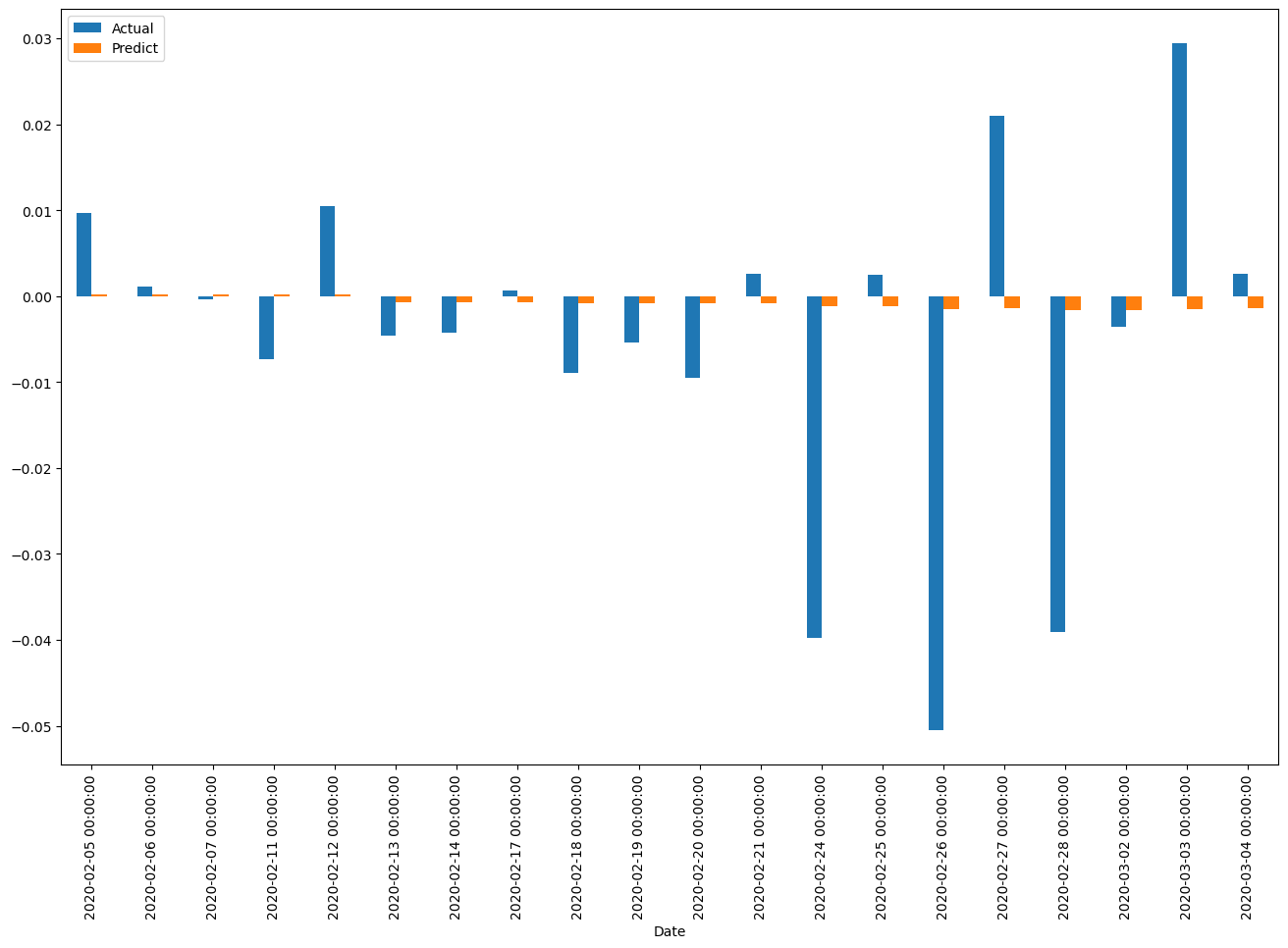
(df_report+1).cumprod().plot()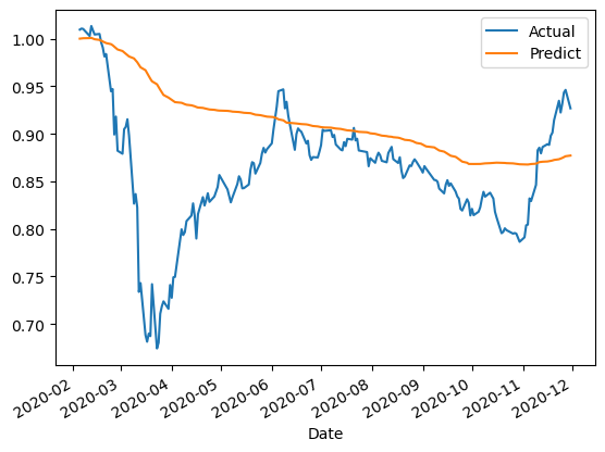
test model with data split
X_live = df1.iloc[1200:]X_live| Prior | Open | High | Low | Close | PE_x | PE_y | EPS | gdp | Return_shift | PE_Label | EPS_Label | GDP_Label | |
|---|---|---|---|---|---|---|---|---|---|---|---|---|---|
| Date | |||||||||||||
| 2020-12-01 | 1408.31 | 1419.28 | 1430.03 | 1416.39 | 1420.87 | 28.11 | 25.9028 | 55.4349 | 3.924572e+12 | 0.008918 | 2 | 3 | 2 |
| 2020-12-02 | 1420.87 | 1416.46 | 1430.49 | 1415.10 | 1417.95 | 28.06 | 25.8395 | 55.3846 | 3.924572e+12 | -0.002055 | 2 | 3 | 2 |
| 2020-12-03 | 1417.95 | 1424.31 | 1439.22 | 1420.69 | 1438.32 | 28.49 | 26.2152 | 38.9297 | 3.924572e+12 | 0.014366 | 2 | 1 | 2 |
| 2020-12-04 | 1438.32 | 1439.14 | 1454.94 | 1439.14 | 1449.83 | 28.73 | 26.4263 | 38.9327 | 3.924572e+12 | 0.008002 | 2 | 1 | 2 |
| 2020-12-08 | 1449.83 | 1447.71 | 1484.73 | 1442.65 | 1478.92 | 29.34 | 26.9521 | 38.9373 | 3.924572e+12 | 0.020064 | 2 | 1 | 2 |
| … | … | … | … | … | … | … | … | … | … | … | … | … | … |
| 2021-10-28 | 1627.61 | 1626.27 | 1632.30 | 1622.56 | 1624.31 | 20.81 | 19.5438 | 83.6187 | 3.997128e+12 | -0.002028 | 1 | 6 | 2 |
| 2021-10-29 | 1624.31 | 1627.01 | 1629.25 | 1619.14 | 1623.43 | 21.02 | 19.5307 | 83.1111 | 3.997128e+12 | -0.000542 | 1 | 6 | 2 |
| 2021-11-01 | 1623.43 | 1627.54 | 1632.73 | 1611.39 | 1613.78 | 20.89 | 19.4140 | 83.1221 | 3.997128e+12 | -0.005944 | 1 | 6 | 2 |
| 2021-11-02 | 1613.78 | 1616.86 | 1621.69 | 1608.64 | 1617.89 | 20.96 | 19.4637 | 83.1246 | 3.997128e+12 | 0.002547 | 1 | 6 | 2 |
| 2021-11-03 | 1617.89 | 1620.90 | 1623.08 | 1607.72 | 1611.92 | 20.87 | 19.3909 | 83.1235 | 3.997128e+12 | -0.003690 | 1 | 6 | 2 |
221 rows × 13 columns
X_live[['EPS','PE_y','gdp','EPS_Label', 'PE_Label','GDP_Label']]| EPS | PE_y | gdp | EPS_Label | PE_Label | GDP_Label | |
|---|---|---|---|---|---|---|
| Date | ||||||
| 2020-12-01 | 55.4349 | 25.9028 | 3.924572e+12 | 3 | 2 | 2 |
| 2020-12-02 | 55.3846 | 25.8395 | 3.924572e+12 | 3 | 2 | 2 |
| 2020-12-03 | 38.9297 | 26.2152 | 3.924572e+12 | 1 | 2 | 2 |
| 2020-12-04 | 38.9327 | 26.4263 | 3.924572e+12 | 1 | 2 | 2 |
| 2020-12-08 | 38.9373 | 26.9521 | 3.924572e+12 | 1 | 2 | 2 |
| … | … | … | … | … | … | … |
| 2021-10-28 | 83.6187 | 19.5438 | 3.997128e+12 | 6 | 1 | 2 |
| 2021-10-29 | 83.1111 | 19.5307 | 3.997128e+12 | 6 | 1 | 2 |
| 2021-11-01 | 83.1221 | 19.4140 | 3.997128e+12 | 6 | 1 | 2 |
| 2021-11-02 | 83.1246 | 19.4637 | 3.997128e+12 | 6 | 1 | 2 |
| 2021-11-03 | 83.1235 | 19.3909 | 3.997128e+12 | 6 | 1 | 2 |
221 rows × 6 columns
X_live| Prior | Open | High | Low | Close | PE_x | PE_y | EPS | gdp | Return_shift | PE_Label | EPS_Label | GDP_Label | |
|---|---|---|---|---|---|---|---|---|---|---|---|---|---|
| Date | |||||||||||||
| 2020-12-01 | 1408.31 | 1419.28 | 1430.03 | 1416.39 | 1420.87 | 28.11 | 25.9028 | 55.4349 | 3.924572e+12 | 0.008918 | 2 | 3 | 2 |
| 2020-12-02 | 1420.87 | 1416.46 | 1430.49 | 1415.10 | 1417.95 | 28.06 | 25.8395 | 55.3846 | 3.924572e+12 | -0.002055 | 2 | 3 | 2 |
| 2020-12-03 | 1417.95 | 1424.31 | 1439.22 | 1420.69 | 1438.32 | 28.49 | 26.2152 | 38.9297 | 3.924572e+12 | 0.014366 | 2 | 1 | 2 |
| 2020-12-04 | 1438.32 | 1439.14 | 1454.94 | 1439.14 | 1449.83 | 28.73 | 26.4263 | 38.9327 | 3.924572e+12 | 0.008002 | 2 | 1 | 2 |
| 2020-12-08 | 1449.83 | 1447.71 | 1484.73 | 1442.65 | 1478.92 | 29.34 | 26.9521 | 38.9373 | 3.924572e+12 | 0.020064 | 2 | 1 | 2 |
| … | … | … | … | … | … | … | … | … | … | … | … | … | … |
| 2021-10-28 | 1627.61 | 1626.27 | 1632.30 | 1622.56 | 1624.31 | 20.81 | 19.5438 | 83.6187 | 3.997128e+12 | -0.002028 | 1 | 6 | 2 |
| 2021-10-29 | 1624.31 | 1627.01 | 1629.25 | 1619.14 | 1623.43 | 21.02 | 19.5307 | 83.1111 | 3.997128e+12 | -0.000542 | 1 | 6 | 2 |
| 2021-11-01 | 1623.43 | 1627.54 | 1632.73 | 1611.39 | 1613.78 | 20.89 | 19.4140 | 83.1221 | 3.997128e+12 | -0.005944 | 1 | 6 | 2 |
| 2021-11-02 | 1613.78 | 1616.86 | 1621.69 | 1608.64 | 1617.89 | 20.96 | 19.4637 | 83.1246 | 3.997128e+12 | 0.002547 | 1 | 6 | 2 |
| 2021-11-03 | 1617.89 | 1620.90 | 1623.08 | 1607.72 | 1611.92 | 20.87 | 19.3909 | 83.1235 | 3.997128e+12 | -0.003690 | 1 | 6 | 2 |
221 rows × 13 columns
live_data =X_live[['EPS','PE_y','gdp','EPS_Label', 'PE_Label','GDP_Label']]live_data['Return_shift']=model.predict(live_data)df_live_report = pd.DataFrame({'Actual': X_live['Return_shift'], 'Predict':live_data['Return_shift']})
df_live_report| Actual | Predict | |
|---|---|---|
| Date | ||
| 2020-12-01 | 0.008918 | 0.000900 |
| 2020-12-02 | -0.002055 | 0.000870 |
| 2020-12-03 | 0.014366 | 0.000208 |
| 2020-12-04 | 0.008002 | 0.000300 |
| 2020-12-08 | 0.020064 | 0.000529 |
| … | … | … |
| 2021-10-28 | -0.002028 | 0.001105 |
| 2021-10-29 | -0.000542 | 0.001075 |
| 2021-11-01 | -0.005944 | 0.001025 |
| 2021-11-02 | 0.002547 | 0.001047 |
| 2021-11-03 | -0.003690 | 0.001015 |
221 rows × 2 columns
df_live_report_exmaple = df_live_report.head(200)
df_live_report_exmaple.plot(kind='bar',figsize=(16,10))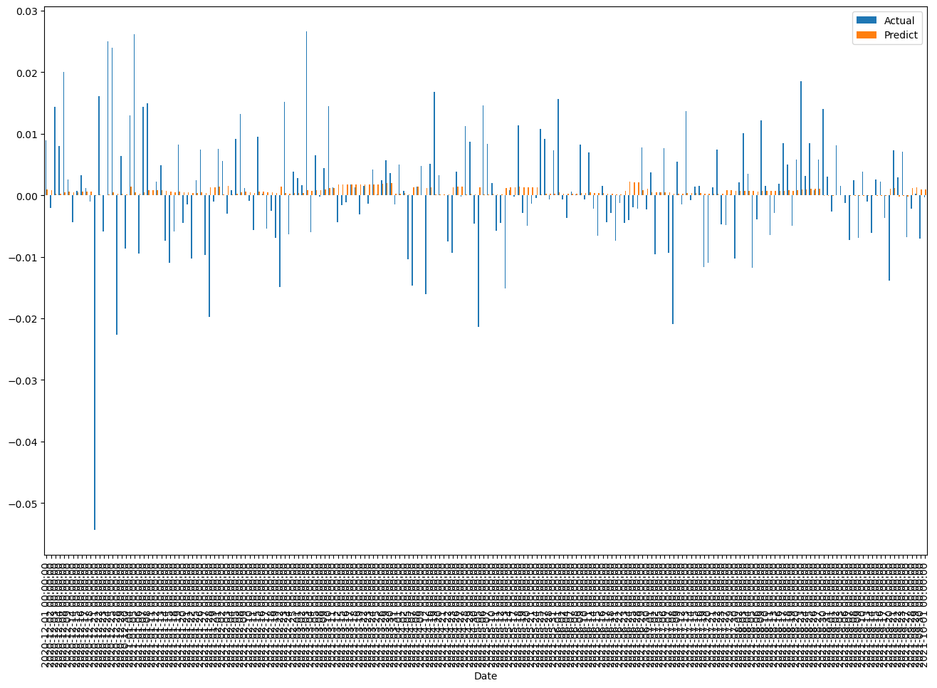
(df_live_report_exmaple).plot()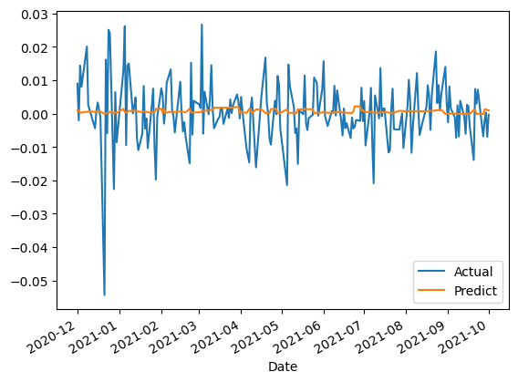
(df_live_report_exmaple+1).cumprod().plot()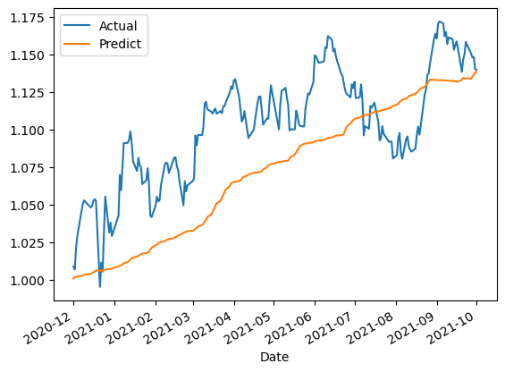
Conclusion
In this article, we demonstrated how to perform stock analysis and predict stock returns using Python. We started by importing and merging multiple datasets,
including historical stock prices, earnings per share (EPS), and GDP data. After merging the datasets and adding stock return calculations, we used linear regression to predict stock returns based on historical data.
We then visualized the results using various libraries like pandas, matplotlib, numpy, and seaborn.
The results showed that our linear regression model provided a reasonable prediction of stock returns, although it is important to note that stock market predictions are inherently uncertain and should not be solely relied upon for investment decisions.
Further improvements to the model could be achieved by incorporating additional variables, using more advanced techniques, or incorporating domain-specific knowledge.
Overall, this article serves as a foundation for further exploration into stock analysis and prediction using Python, providing valuable insights for investors and analysts looking to harness the power of data-driven decision-making.